Navigating big simulations
Visualisation of big data is a navigation problem
This post is based on my AIAA Scitech 2026 paper, which you can also find here. The code is here.
Visualisation is the communication channel between raw data and our principal means of interpretation and synthesis - our brain! In looking at visual representations, we are seeking confirmation, one way or another, of the validity of our ideas. The goal is visualisation at the speed of thought.
The challenge is that we regularly work with datasets that require an HPC system to keep in memory and take many minutes (at least) to transfer to persistent storage.
This post describes two related techniques to tackle this problem. Extract-tiles applies 3D tiling (hierarchical level of detail) to 3D surfaces obtained from our simulations - this allows us to navigate our results interactively on any device. Linked views enables us to synchronise different plots so we can see the effect of a particular feature from several perspectives in our data - allowing us to synthesise multiple data channels into a new finding.
Connecting effect to cause
The video at the start of this post shows a computational fluid dynamics (CFD) simulation of a compressor during a stall event. This is a 4D problem - the simulation has approximately 150 million grid points and is also evolving in time. Since the 1990s, experimental data, like the line traces of pressure vs time shown in the video, have been measured and the signature of stall recorded, but the cause — what is happening in the flow to produce these measurements — remained unknown until a group of us used CFD to dig deeper. The findings were first presented in 2012 and I worked on connecting line traces to the flow field; it was a laborious process involving lots of python scripts and files. It certainly was not interactive!
The video shows how extract-tiles and linked views solve this problem. The pressure traces and the two 3D views are connected: moving the red vertical lines changes the time, and moving the horizontal lines changes the circumferential position of the camera. We can see a perturbation in the line traces and immediately, interactively, view the flow that is responsible. Navigation to the right place, at the right time, is key to enabling us to connect cause and effect.
A live demo of extract-tiles
The live demo below focus on the extract-tile rendering of the compressor. As you zoom and rotate, different parts of the machine are loaded and shown at different levels of detail; the time snapshot is controlled by a slider in the dropdown GUI.
The surfaces in this snapshot are the blades, the hub geometry, and an iso-surface at zero axial velocity. The iso-surface highlights regions of reversed flow and is a useful diagnostic during stall. Each snapshot is represented using five levels of tiles. For each snapshot, the finest level contains more than 1500 tiles and 20 million triangles.
From extracts to extract-tiles
To make the storage problem tractable, CFD users often only retain subsets, “extracts”, of the raw data. For our purposes, we take extracts to mean 3D surfaces, but 2D surfaces, or 1D lines, or even 0D values are also extracts.
The key observation is that a 3D surface, viewed from any given camera position, may contain more data than we can visualise (more data points than we have pixels). This issue was first highlighted by James H. Clark in a paper in 1976,
It makes no sense to use 500 polygons in describing an object if it covers only 20 raster units of the display.
One answer, which we adopt here, is to store the surface at multiple levels of detail and in different spatial chunks. Each piece is a separate file (or “tile”) with the objective that each tile be the same size (on disk). A zoomed-out view of a large region and a zoomed-in view of a small region should each need roughly the same amount of data. Sound familiar? This is exactly how online mapping works.
The tile building process is done offline, as a pre-processing step, so that all the tiles are ready-to-go at visualisation-time. The bounding cuboid volume is divided using an octree (each cell has 8 child cells, recursively). The mesh of triangles that lie within a tile (or that span the tile’s boundary) is then simplified (vertices are removed) until the target file size is reached. For this decimation process, we use the quadric error metrics approach of Garland and Heckbert. At the finest level (the leaf nodes of the octree), the original triangles are retained.
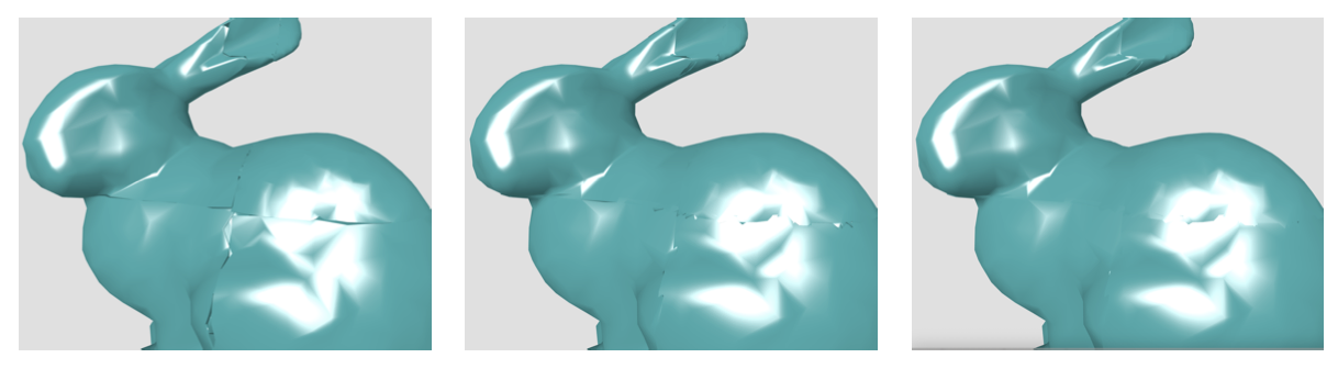
We need to take a little care to avoid “cracks” at tile boundaries (left picture). The current implementation creates a small overlap, or “flange” (middle picture), of vertices whose location is snapped back on to the original mesh surface (right picture).
The extract-tiles are rendered in the browser using three.js. Using a list of available tiles that includes the average edge length of the triangles in each tile, the viewer fetches only the tiles that are currently needed. A proxy for Screen Space Error (SSE) is derived by obtaining the approximate number of pixels needed to cover the average edge length when projected on to the screen in the current view. If the SSE is above a pre-set threshold, the children of the current tile are fetched; if it is below another threshold, the parent tile is loaded and its children are expunged.
Linked views
Tiling is critical to interactive delivery, but linked views are key to accelerating interpretation.
dbslice is used as a convenient web-based framework for multiple interactive plots. dbslice allows dimensions, such as time or circumferential position, to be registered, shared, manipulated and consumed. Changing a dimension in one plot can be configured to update an extract-tile plot by changing either the data (e.g. responding to the time dimension by fetching new time snapshots) or the view (e.g. responding to the circumferential position dimension by changing the camera position).
The analysis experience, and hence our ability to derive new findings, is completely transformed from a slow, manual manipulation of files into an interactive collection of synchronised, dynamic visualisations.
Implementation
Starting from a source GLB mesh, such as one exported from ParaView, the tile builder partitions the geometry into a multi-resolution hierarchy and writes a manifest JSON plus the individual tile payloads as GLB files. The tile builder is written in Python, using trimesh for GLB parsing and mesh subsetting and Open3D for quadric error mesh simplification.
The viewer is written in JavaScript on top of three.js. It performs frustum culling and screen-space-error based level-of-detail selection in plain client-side code, then streams manifests and tiles on demand and keeps a small in-memory cache of recently used tiles.